Correction of spectra
Loading functions:
import h5py
import numpy as np
import matplotlib.pyplot as plt

def load_runs(runs,bt):
    '''
    Load hdf5-file from runs, containing
        (x,y) coordinates of droplets [dim ndroplets]
        intensity of droplets         [dim ndroplets]
        number of droplets            [dim nshots]
        intensity of pulses           [dim nshots]

    Call: x,y,adi,ndrop,gmd = load_runs([run1,run2,...],bt)
    '''
    x = []; y = []; adu = []; ndrop = []; gmd = []
    for run in runs:
        if bt == 'instruction':
            fh = h5py.File('../../example_data/run-%03d.h5' %run, 'r')
            X  = fh['x'][()]; Y = fh['y'][()]; I = fh['adu'][()]
            N  = fh['ndroplets'][()]; E = fh['pulse_energy'][()]
            fh.close()
        x.append(X); y.append(Y); adu.append(I),ndrop.append(N); gmd.append(E)
    return np.concatenate(x),np.concatenate(y),np.concatenate(adu),np.concatenate(ndrop),np.concatenate(gmd)

def det_geom(img,bt):
    '''
    Correct image for detector geometry
    '''
    if bt == 'instruction':
        new_img = [];  I = 0
        for i in np.arange(709):
            if (i > 352) and (i < 358):  new_img.append(np.zeros(len(img[0])+5))
            else:
                tmp = img[I]
                for j in np.arange(5): tmp = np.insert(tmp, 384, 0.0)
                new_img.append(tmp); I += 1
    return new_img

def create_img_v1(x,y,adu,ndrop,adu_int,scale_signal):
    '''
    Version 1 of a script which creates the full image

    Call: img = create_img_v1(x,y,adu,ndrop,adu_interval,scale_signal)
    '''
    ind, = np.where((adu >= adu_int[0]) & (adu <= adu_int[1]))
    if scale_signal == True:    img, xedges, yedges = np.histogram2d(x[ind], y[ind], bins=[np.arange(705), np.arange(769)],weights=adu[ind])
    elif scale_signal == False: img, xedges, yedges = np.histogram2d(x[ind], y[ind], bins=[np.arange(705), np.arange(769)])
    det_geom(img,'instruction')
    return img

def create_img(x,y,adu,ndrop,adu_int,scale_signal):
    '''
    Create image with some ADU signals

    Call: img = create_img_v1(x,y,adu,ndrop,adu_interval,scale_signal)
    '''
    ind, = np.where((adu >= adu_int[0]) & (adu <= adu_int[1]))
    if scale_signal == True:    img, xedges, yedges = np.histogram2d(x[ind], y[ind], bins=[np.arange(705), np.arange(769)],weights=adu[ind])
    elif scale_signal == False:
        img_1ph, xedges, yedges = np.histogram2d(x[ind], y[ind], bins=[np.arange(705), np.arange(769)])
        ind, = np.where((adu >= 2.0*adu_int[0]) & (adu <= 2.0*adu_int[1]))
        img_2ph, xedges, yedges = np.histogram2d(x[ind], y[ind], bins=[np.arange(705), np.arange(769)])
        img = img_1ph + 2.0*img_2ph # scale 2-photon image by factor 2
    det_geom(img,'instruction')
    return img

def plot_raw(runs,roi,adu_int,plot_results,bt):
    '''
    Plot histogram, detector image, and projections
    Can include an ROI or do this over full image

    Call: spat_spec,xes_spec = plot_raw(runs,roi,adu_int,plot_results,bt)
    '''
    x,y,adu,ndrop,gmd = load_runs(runs,bt)
    print('Looking at runs {}-{} from expt \'{}\', with {:.2e} shots and {:.2e} droplets.'.format(runs[0],runs[len(runs)-1],bt,len(ndrop),sum(ndrop)))
    img = create_img(x,y,adu,ndrop,adu_int,False)
    spat_spec = np.sum(img, axis=0)/len(ndrop)
    xes_spec  = np.sum(img, axis=1)/len(ndrop)

    if plot_results == True:
        plt.figure(figsize=(16,4))
        plt.subplot(141); plt.title('Detector image')
        vmin, vmax = np.percentile(img, [1, 99])
        plt.imshow(img, origin='lower',vmin=vmin, vmax=vmax,aspect='auto')
        if roi != False:
            plt.plot([roi[2],roi[2]],[roi[0],roi[1]],'w--')
            plt.plot([roi[3],roi[3]],[roi[0],roi[1]],'w--')
            plt.xlim((0,len(img[0]))); plt.ylim((0,len(img)))
        plt.subplot(142); plt.title('Spatial projection')
        plt.plot(spat_spec,'b')
        plt.plot([roi[2],roi[2]],[0,max(np.sum(img, axis=0)/len(ndrop))],'r--')
        plt.plot([roi[3],roi[3]],[0,max(np.sum(img, axis=0)/len(ndrop))],'r--')
        plt.xlim((roi[2]-50,roi[3]+50))
        plt.ylabel('Signal / no. shots')
        plt.subplot(143); plt.title('Energy-dispersive projection')
        plt.plot(xes_spec,'b')
        plt.ylabel('Signal / no. shots')
        plt.subplot(144); plt.title('Histogram')
        ind, = np.where((y >= roi[2]) & (y <= roi[3]))
        p = np.percentile(adu[ind], 99.9) # 99.9th percentile, for xmax
        hist, bin_edges = np.histogram(adu[ind],bins = np.arange(0,p,p/500.))
        ylims = [0.0001*np.max(hist),1.1*np.max(hist)]
        plt.plot([adu_int[0],adu_int[0]],ylims,'-',color='r')
        plt.plot([adu_int[1],adu_int[1]],ylims,'-',color='r')
        plt.plot(bin_edges[1:]-0.5,hist,'b'); plt.yscale('log')
        plt.tight_layout()
    return spat_spec,xes_spec
Load raw image which is to be:
Corrected for background signal
Corrected for detector gap
Given the energy axis
runs    = [1]
adu_int = [97.0,123.0]
roi     = [0,705,310,348]
bt      = 'instruction'
adu_int = [97.0,123.0]
x,y,adu,ndrop,gmd = load_runs(runs,bt)
img = create_img(x,y,adu,ndrop,adu_int,False)
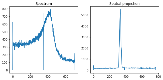
Without any corrections, the spectrum and spatial projection looks as follows:
plt.figure(figsize=(8,4))
plt.subplot(121); plt.title('Spectrum')
xes_spec  = np.sum(img, axis=1)
plt.plot(xes_spec)

plt.subplot(122); plt.title('Spatial projection')
spat_spec = np.sum(img, axis=0)
plt.plot(spat_spec)
plt.tight_layout(); plt.show()
Background correction
The first correction we will discuss is the removal of background signal, or noise. With the ADU interval selected, noise due to thermal signal is removed, and remaining noise is largely due to elastic scattering, and if the shielding is appropriate this will likely be relatively low and quite homogenous over the detector. The protocols discussed here will work best for this scenario, and, e.g., a background signal with a hotspot that is in the vicinity of the inelastic signal will be harder to consider with these approaches.
Pulling down to zero
The most straight-forward background subtraction is to simply bring the signal at some defined part of the spectrum down to zero (or any desired value). Here we illustrate this by putting the 600-650 pixel region to zero:
# bring to zero
#
#
This approach is straightforward, but it suffers from a number of issues:
Assuming that the physical signal is zero in this region, thus disregarding any spectrum tails which will overlap with this region
Assuming that the background signal is homogenous over the entire spectrum region, which is quite unlikely.
It will result in negative signal at some energies, which is physically incorrect.
Remove footprint
Another approach is to take the signal footprint at some other part of the detector and subtract this from the ROI:
# remove footprint
#
#
This again has some issues:
While it doesn’t require the background signal to be homogenous over the energy-dispersive direction, it need it to be relatively homogenous over the spatial direction.
It requires that the detector corretions (especially the gain) is accurate. This assumption is hard to avoid and is present in the other corrections as well, but it is particularly present here.
Raw-by-raw interpolation
Instead of taking the footprint at one side of the ROI (or potentially both sides), an alternative is to perform a row-by-row interpolation of the background signal over the ROI region. This requires the definition of the ROI as well as the interpolation region, and interpolation can use, e.g., polynomials of arbitrary order.
Define the interpolation region. This should preferably be a relatively flat region of the spatial projection, and not contail any significant signal tails from the spectrometer crystals.
# interpolation region
Interpolate using polynomial of desired order
def remove_background_order(img, a, b, c, d, o):
    x = np.concatenate((np.arange(a, b), np.arange(c, d)))
    img_corrected = np.copy(img)
    for i in range(img.shape[0]):
        y = np.concatenate((img[i, a:b], img[i, c:d]))
        poly = np.poly1d(np.polyfit(x, y, o))
        img_corrected[i, :d] = img[i, :d] - poly(np.arange(d))
    return img_corrected

fit = [284,304,358,378]

raw_spec = np.sum(img[roi[0]:roi[1]:,roi[2]:roi[3]], axis=1)
zer_spec = np.sum(remove_background_order(img, fit[0], fit[1], fit[2], fit[3],0)[roi[0]:roi[1]:,roi[2]:roi[3]], axis=1)
one_spec = np.sum(remove_background_order(img, fit[0], fit[1], fit[2], fit[3],1)[roi[0]:roi[1]:,roi[2]:roi[3]], axis=1)
two_spec = np.sum(remove_background_order(img, fit[0], fit[1], fit[2], fit[3],2)[roi[0]:roi[1]:,roi[2]:roi[3]], axis=1)
thr_spec = np.sum(remove_background_order(img, fit[0], fit[1], fit[2], fit[3],3)[roi[0]:roi[1]:,roi[2]:roi[3]], axis=1)

plt.figure(figsize=(10,4))
plt.subplot(121)
plt.plot(raw_spec); plt.plot(one_spec); plt.plot(raw_spec-one_spec)
plt.legend(('Raw','Corr','diff'))

plt.subplot(122)
plt.plot(raw_spec-zer_spec); plt.plot(raw_spec-one_spec+50)
plt.plot(raw_spec-two_spec+100); plt.plot(raw_spec-thr_spec+150)
plt.plot([0,705],[0,0],'k--',zorder=1);     plt.plot([0,705],[50,50],'k--',zorder=1)
plt.plot([0,705],[100,100],'k--',zorder=1); plt.plot([0,705],[150,150],'k--',zorder=1)
plt.legend(('0:th','1:st','2:nd','3:rd'),ncol=4)
plt.yticks([0,25,50,75,100,125,150,175,200],[])
plt.xlim((0,705)); plt.ylim((-10,220))
plt.tight_layout(); plt.show()
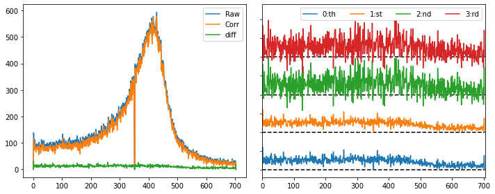
In this case we see that a 2:nd or 3:rd order polynomial yields large fluctuation, as the background is quite noisy and the interpolation can thus be a bit overfitted. Our experiences are that a first-order fit is most stable, and as such xest has the following as default background subtraction function:
def remove_background(img, a, b, c, d):
    x = np.concatenate((np.arange(a, b), np.arange(c, d)))
    img_corrected = np.copy(img)
    for i in range(img.shape[0]):
        y = np.concatenate((img[i, a:b], img[i, c:d]))
        poly = np.poly1d(np.polyfit(x, y, 1))
        img_corrected[i, :d] = img[i, :d] - poly(np.arange(d))
    return img_corrected
We acknowledge that this function is not perfect, and it can have problems in particular with:
Noisy signal
Diagonally spread background, as this assumes relative homogenuity in the spatial direction
One possibility that could account for noisy signal as well as some diagonal signal is to account for the signal for neighbouring rows in the interpolation. We refrain from doing so as a standard.
Interpolating over detector gap
Depending on the detector used, it is possible that there will be a gap between detector plates which will lead to a region without any detected signal. In the data considered here, an epix100 detector with 4 panels was used, leading to gaps in both the spatial and energy-dispersive direction.
The gap in the spatial direction can (and most definitely should) be avoided by moving the detector, and it should be placed in such a matter that it doesn’t interfer with any background correction scheme. The gap in the energy-dispersive direction is often more difficult to remove, as the spectrum region resolved may be rather extensive, and the detector position can be limited by other components of the experimental set-up. As such, a scheme of interpolating over this gap can be applied, and we here favour a second-order polynomial fitted of over it:
# interpolation
#
#
def interpolate_epix_gap(spectrum,bt):
    if (bt == 'LR81'):
        a, b = 309, 349; c, d = 361, 401
    xaxis = np.arange(spectrum.shape[0])
    x = np.concatenate((xaxis[a:b], xaxis[c:d]))
    y = np.concatenate((spectrum[a:b], spectrum[c:d]))
    poly = np.poly1d(np.polyfit(x, y, 2))
    spectrum[b:c] = poly(xaxis[b:c])
Here a region for fittin has to be decided, as well as the order of the polynomial. Our experiences is that the above combination is most suitable for our experiments, but other schemes may be more appropriate. Note that any interpolation can only be approximate, and should be done with some care. Ideally, the gap should be far away from the peak max, in order to minimize any potential artifact from interfering with the main spectrum region of interest.
Note
If the detector image has to be rotated, the interpolation region must include all parts of the projected spectrum which overlaps with any part of the gap. This means that it may be appropriate to add a few extra pixels, as it can be hard to judge if one pixel has a lower signal due to rotation, or just as a result of the general noise.
Energy calibration
Ensuring correct vertical and horizontal distances between the sample, spectrometer, and detector will typically only work so far, so additional fine-tuning will be needed. For the measurements described here, calibration is primarily done by use of reference samples (MnCl\(_2\)), as well as by ensuring good correspondance between the 0F spectra collected over different beamtimes. The latter is largely added as only using reference samples yield a number of parameters which works approximately equally well, and adding the 0F will narrow down the potential combinations more.
With a von Hamos spectrometer, the calibration is decided by the lattice constant of the crystal, horizontal/vertical (depending on beam polarization) set-off A, and radius of the spectrometer R. Furthermore, the pixel size is needed. With this, the calibration of the experiment discussed is is given as:
# energy calibration
#
#
def energy_axis(A,R,bt):
    d = 0.9601
    if (bt == 'instruction'):
        pix = 0.05; l = np.arange(709).astype(np.float64)
    l *= pix
    ll = l/2 - (np.amax(l) - np.amin(l)) / 4
    factor = 1.2398e4
    xaxis = factor / (2.0*d*np.sin(np.arctan(R/(ll + A))))
    return xaxis

axis_para = [50.72,498.21]

# left: spectrum without energy

# left: spectrum with energy
Producing corrected spectra
A function for producing the final spectrum is thus provided. This will use:
A first-order row-by-row background correction
A second-order gap interpolation
Furthermore, it can either provide an energy-axis in eV or pixel number, and it can plot the resulting projections if so desired.
def proj_spectrum(runs,roi,fit,adu_int,axis_para,thr,plot_proj,bt):
    if axis_para == False:
        xaxis = False
    else:
        xaxis = energy_axis(axis_para[0],axis_para[1],bt)
    if thr == False:
        x,y,adu,ndroplets,gmd = load_runs(runs,bt)
        print 'Looking at data from beamtime',bt,'with',len(ndroplets),'shots.'
        img,vmin,vmax = create_img(runs,x,y,adu,adu_int,adu_int[2],bt)
        if bt == 'LV30':
            img[:400,:] = 0.0
        elif bt == 'LS10':
            img[550:,:] = 0.0; img[:,:150] = 0.0; img[:,250:] = 0.0
        cor_spec = np.sum(remove_background(img, fit[0], fit[1], fit[2], fit[3])[:,roi[0]:roi[1]], axis=1)
        interpolate_epix_gap(cor_spec,bt)
        if plot_proj:
            tmp_spat = np.sum(img, axis=0)
            cor_spat = np.sum(remove_background(img, fit[0], fit[1], fit[2], fit[3]), axis=0)
            tmp_spec = np.sum(img[:,roi[0]:roi[1]], axis=1)
    else:
        x,y,adu,ndroplets,gmd,rej,hitinfo = HitFinder(runs,thr,roi,fit,adu_int,False,bt)
        img,vmin,vmax = create_img(runs,x,y,adu,adu_int,adu_int[2],bt)
        if bt == 'LV30':
            img[:400,:] = 0.0
        elif bt == 'LS10':
            img[550:,:] = 0.0; img[:,:150] = 0.0; img[:,250:] = 0.0
        cor_spec = np.sum(remove_background(img, fit[0], fit[1], fit[2], fit[3])[:,roi[0]:roi[1]], axis=1)
        interpolate_epix_gap(cor_spec,bt)
        if plot_proj:
            x_all,y_all,adu_all,ndroplets_all,gmd_all = load_runs(runs,bt)
            img_all,vmin,vmax = create_img(runs,x_all,y_all,adu_all,adu_int,adu_int[2],bt)
            cor_spat = np.sum(img, axis=0)
            tmp_spat = np.sum(img_all, axis=0)
            tmp_spec = np.sum(remove_background(img_all, fit[0], fit[1], fit[2], fit[3])[:,roi[0]:roi[1]], axis=1)
            interpolate_epix_gap(tmp_spec,bt)
    if plot_proj:
        fig = plt.figure(figsize=(12,3))
        ################
        plt.subplot(141); plt.title('Detector image',fontsize=9)
        plt.imshow(img, origin='lower',vmin=vmin, vmax=vmax,aspect='auto')
        plt.plot([roi[0],roi[0]],[roi[2],roi[3]],'w-'); plt.plot([roi[1],roi[1]],[roi[2],roi[3]],'w-')
        plt.plot([fit[0],fit[0]],[roi[2],roi[3]],'w--');plt.plot([fit[1],fit[1]],[roi[2],roi[3]],'w--')
        plt.plot([fit[2],fit[2]],[roi[2],roi[3]],'w--');plt.plot([fit[3],fit[3]],[roi[2],roi[3]],'w--')
        plt.xlim((fit[0]-20,fit[3]+20))
        plt.ylim((roi[2],roi[3]))
        plt.xticks(fontsize=8); plt.yticks(fontsize=9)
        ################
        plt.subplot(142); plt.title('Spatial projection',fontsize=9)
        plt.plot(tmp_spat/len(ndroplets))
        plt.plot(cor_spat/len(ndroplets),'r')
        plt.plot((tmp_spat-cor_spat)/len(ndroplets),'k')
        ylims = [0,0.8*max(tmp_spat)/len(ndroplets)]
        plt.plot([roi[0],roi[0]],ylims,'g');  plt.plot([roi[1],roi[1]],ylims,'g')
        plt.plot([fit[0],fit[0]],ylims,'g--');plt.plot([fit[1],fit[1]],ylims,'g--')
        plt.plot([fit[2],fit[2]],ylims,'g--');plt.plot([fit[3],fit[3]],ylims,'g--')
        plt.xlim((fit[0]-20,fit[3]+20))
        plt.ylim((0,1.05*max(tmp_spat)/len(ndroplets)))
        plt.xticks(fontsize=9); plt.yticks(fontsize=9)
        plt.ylabel('Signal / no. shots',fontsize=9)
        ################
        plt.subplot(143); plt.title('Spectrum',fontsize=9)
        if axis_para == False:
            plt.plot(tmp_spec/len(ndroplets))
            plt.plot(cor_spec/len(ndroplets),'r')
            plt.plot((tmp_spec-cor_spec)/len(ndroplets),'k')
        else:
            plt.plot(xaxis,tmp_spec/len(ndroplets))
            plt.plot(xaxis,cor_spec/len(ndroplets),'r')
            plt.plot(xaxis,(tmp_spec-cor_spec)/len(ndroplets),'k')
            plt.xlim(6480,6500)
        if thr == False: plt.legend(('Raw','Corr.','Bkgrd'),fontsize=9,loc='upper left')
        else:            plt.legend(('All','Hits','Diff.'),fontsize=9,loc='upper left')
        plt.ylabel('Signal / no. shots',fontsize=9)
        plt.ylim((0,1.05*max(tmp_spec)/len(ndroplets)))
        plt.xticks(fontsize=9); plt.yticks(fontsize=9)
        ################
        plt.subplot(144); plt.title('Final spectrum',fontsize=9)
        if axis_para == False:
            plt.plot(cor_spec,'r')
        else:
            plt.plot(xaxis,cor_spec,'r')
            plt.xlim(6480,6500)
        plt.ylabel('Total intensity [counts]',fontsize=9)
        plt.ylim((0,1.05*max(cor_spec)))
        plt.xticks(fontsize=8); plt.yticks(fontsize=9)
        ################
        plt.tight_layout()
    return xaxis,cor_spec
  File "<ipython-input-11-18c3fe161a39>", line 8
    print 'Looking at data from beamtime',bt,'with',len(ndroplets),'shots.'
                                        ^
SyntaxError: invalid syntax
Signal interval and multi-photon hits
With this, we now return to the question of adopted signal interval and multi-photon hits:
adu_ints = [[102.0,117.0],[97.0,123.0],[92.0,128.0]]
for adu_int in adu_ints:
    spat_spec,xes_spec = plot_raw(runs,roi,adu_int,False,bt)
    ax0.plot(spat_spec/sum(spat_spec))
    ax1.plot(xes_spec/sum(xes_spec))

proj_spectrum_v1
if axis_para == False:
    xaxis = False
else:
    xaxis = energy_axis(axis_para[0],axis_para[1],bt)

check with different ADU intervals
Note that the difference…
And for multi-photon hits:
Incling two-photon hits here seems to work well enough.